Unconstrained MPC regulator with Kalman filter

Table of Contents

Unconstrained Model Predictive Control (MPC) regulator with Kalman filter¶

The following presents an unconstrained Linear Quadratic Model Predictive Control (LQ-MPC) simulation using Matlab-kernel for Jupyter Notebook. The code files can be used in Matlab natively.

Pre-requisites¶

• Knowledge in Control Systems theory.
• Convex quadratic optimization theory.
• Jupyter Notebook with Matlab-kernel.
• Matlab.

Background Theory¶

MPC is an optimization-based control strategy that solves a Finite-Horizon Linear Quadratic (FH-LQ) problem subject to constraints. A model of predicted states based on the system dynamics is used to minimize an objective function that satisfies constraints given the actual state. The obtained solution is a sequence of open-loop controls from which only the first one is implemented on the system, inducing feedback. The rest of the sequence is discarded and the process is repeated for the next sampling time, this method is often called Receding-Horizon (RH) principle. Advantages of MPC against other control strategies are the handling of constraints, and non-linearities.

Unconstrained MPC¶

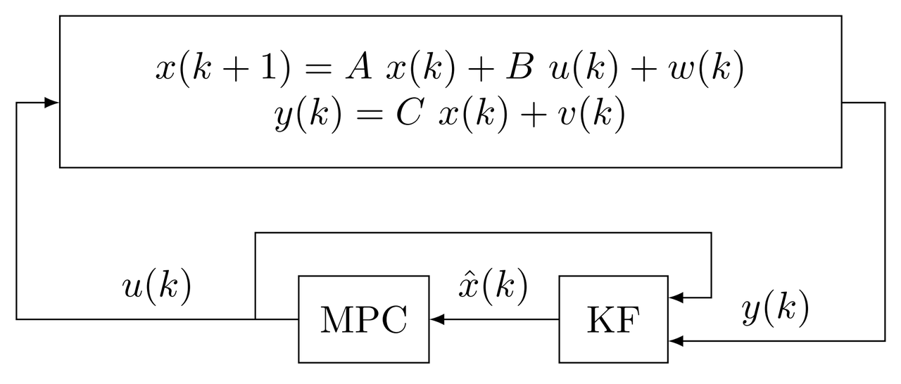
Consider the following discrete-time LTI state-space system, \begin{equation*} \begin{aligned} x(k+1) &= A~x(k)+B~u(k)+w(k)\\ y(k) &= C~x(k)+v(k),\quad k=0,1,2,\dots \end{aligned} \end{equation*} where $x\in\mathbb{R}^n$, $u\in\mathbb{R}^m$, and $y\in\mathbb{R}^p$, are the states, input, and output vectors respectively. $A,~B,~C,$ are the state, input, and output matrices. $A,~B,~C$ are known, no uncertainties in the model, disturbances, and noise. $x(k)$ is available at each sampling time $k$. The process noise is $w(k)\sim \mathcal{N}(0,Q_w)$ with covariance $Q_w$, the measurement noise is $v(k)\sim \mathcal{N}(0,R_v)$ with covariance $R_v$, both are uncorrelated, and are in the form of Additive White Gaussian Noise (AWGN).

Problem Formulation¶

The objective is to regulate $x\rightarrow 0$ as $k\rightarrow \infty$ while minimizing the following cost function,

\begin{align*}\tag{1} J_N(x(k),\mathbf{u}(k)) &= \sum_{j=0}^{N-1} \left( \|x(k+j|k)\|^2_Q + \|u(k+j|k)\|^2_R \right) + \|x(k+N|k)\|^2_P \\ &= \sum_{j=0}^{N-1} (x^\intercal(k+j|k)~Q~x(k+j|k)+ u^\intercal(k+j|k)~R~u(k+j|k) ) + x^\intercal(k+N|k)~P~x(k+N|k) \end{align*}

subject to,

\begin{align*}\tag{2} x(k+1+j|k) &= A~x(k+j|k)+B~u(k+j|k) \\ x(k|k) &= x(k) \end{align*}

for $ j=0,1,2,\dots,N-1$.

Where $Q\in\mathbb{R}^{n\times n}$ and $R\in\mathbb{R}^{m\times m}$ are the state penalty, and input penalty matrices. $P\in\mathbb{R}^{n\times n}$ is the terminal cost matrix, $N \in\mathbb{N}$ is the horizon length, $k$ is the sampling time, and $(k+j|k)$ can be defined as the next $(k+j)$ value given $k$.

With the value function defined as, \begin{align*} J^*_N(x(k),\mathbf{u}(k)) &= \min_{u(k)}~ J_N(x(k),\mathbf{u}(k)) \end{align*} the optimal control sequence is, \begin{equation*} \begin{aligned} \mathbf{u}^*(k) &= \mathrm{arg}\min_{u(k)}~ J^*_N(x(k),\mathbf{u}(k))\\ &= \left\{ u^*(k|k),u^*(k+1|k),\dots,u^*(k+N-1|k) \right\} \end{aligned} \end{equation*}

The Quadratic Problem (QP) approach¶

It's divided in four sections

• Prediction
• Optimization
• Receding Horizon
• Stability

Prediction: Predicted Equality Constraint¶

Setting $x(k)=x(k|k)$, and $u(k)=u(k|k)$ and applying the model recursively,

\begin{align*} x(k+1|k) &= A~x(k)+B~u(k) \\ x(k+2|k) &= A~x(k+1|k)+B~u(k+1|k) \\ &= A^2~x(k)+AB~u(k|k)+B~u(k+1|k) \\ \vdots \hspace{2em} &= \hspace{3em} \vdots \\ x(k+N|k) &= A~x(k+N-1|k)+B~u(k+N-1|k) \\ &= A^N~x(k)+A^{N-1}B~u(k|k)+\dots+B~u(k+N-1|k) \end{align*}

stacking,

\begin{align*} {\underbrace{ \begin{bmatrix} x(k+1|k) \\ x(k+2|k) \\ \vdots \\ x(k+N|k) \end{bmatrix}}_{\mathbf{x}(k)} } = {\underbrace{ \begin{bmatrix} A \\ A^2 \\ \vdots \\ A^N \end{bmatrix}}_{F} } + {\underbrace{ \begin{bmatrix} B & 0 & \dots & 0 \\ AB & B & \dots & 0 \\ \vdots & \vdots & \ddots & \vdots \\ A^{N-1}B & A^{N-2}B & \dots & B \end{bmatrix}}_{G} } {\underbrace{ \begin{bmatrix} u(k|k) \\ u(k+1|k) \\ \vdots \\ u(k+N-1|k) \end{bmatrix}}_{\mathbf{u}(k)} } \end{align*}

the predicted equality constraint is,

\begin{equation}\tag{3} \mathbf{x}(k) = F~x(k)+G~\mathbf{u}(k) \end{equation}

where $\mathbf{x}(k)$, and $\mathbf{u}(k)$ are the state, and input predictions over all steps $j=0,1,2,\dots,N$.

Prediction: Rewriting the Cost Function¶

Rewriting the cost function as,

\begin{aligned} x^\intercal(k|k)~Q~x(k|k) &+ \begin{bmatrix} x(k+1|k) \\ x(k+2|k) \\ \vdots\\ x(k+N|k) \\ \end{bmatrix}^\intercal {\underbrace{ \begin{bmatrix} Q & 0 & \dots & 0 \\ 0 & Q & \ddots & \vdots \\ \vdots & \ddots & Q & 0 \\ 0 & \dots & 0 & P \end{bmatrix}}_{\tilde{Q}} } \begin{bmatrix} x(k+1|k) \\ x(k+2|k) \\ \vdots\\ x(k+N|k) \\ \end{bmatrix} \\ &+ \begin{bmatrix} u(k|k) \\ u(k+1|k) \\ \vdots \\ u(k+N-1|k) \end{bmatrix}^\intercal {\underbrace{ \begin{bmatrix} R & 0 & \dots & 0 \\ 0 & R & \ddots & \vdots \\ \vdots & \ddots & R & 0 \\ 0 & \dots & 0 & R \end{bmatrix}}_{\tilde{R}} } \begin{bmatrix} u(k|k) \\ u(k+1|k) \\ \vdots \\ u(k+N-1|k) \end{bmatrix} \end{aligned}

Therefore, with $x(k|k)=x(k)$, now the problem is to minimize,

\begin{align}\tag{4} J_N(x(k),\mathbf{u}(k)) &= x^\intercal(k)~Q~x(k) + \mathbf{x}^\intercal(k)~\tilde{Q}~\mathbf{x}(k) + \mathbf{u}^\intercal(k)~\tilde{R}~\mathbf{u}(k) \end{align}

subject to,

\begin{align*} \mathbf{x}(k) &= F~x(k)+G~\mathbf{u}(k) \end{align*}

Substituting the predicted equality constraint (3) into the Cost Function (4)¶

Omitting $(k)$ only for the algebraic operations, \begin{align*} J_N(x(k),\mathbf{u}(k)) &= x^\intercal(k) Q x(k) + ( F x(k)+G \mathbf{u}(k) )^\intercal \tilde{Q} ( F x(k)+G \mathbf{u}(k) ) + \mathbf{u}^\intercal(k)~\tilde{R} \mathbf{u}(k) \\ &= x^\intercal Q x + [(F x)^\intercal+(G \mathbf{u})^\intercal] \tilde{Q} (F x+G \mathbf{u}) + \mathbf{u}^\intercal \tilde{R} \mathbf{u} \\ &= x^\intercal Q x + (F x)^\intercal \tilde{Q} F x + (F x)^\intercal \tilde{Q} G \mathbf{u} + (G \mathbf{u})^\intercal \tilde{Q} F x + (G \mathbf{u})^\intercal \tilde{Q} G \mathbf{u} + \mathbf{u}^\intercal~\tilde{R} \mathbf{u}\\ &= \underbrace{x^\intercal Q x + x^\intercal F^\intercal \tilde{Q} F x} + \underbrace{x^\intercal F^\intercal \tilde{Q} G \mathbf{u} + \mathbf{u}^\intercal G^\intercal \tilde{Q} F x} + \underbrace{\mathbf{u}^\intercal G^\intercal \tilde{Q} G \mathbf{u} + \mathbf{u}^\intercal \tilde{R} \mathbf{u}}\\ &= x^\intercal(Q+F^\intercal \tilde{Q} F)x \quad \!\!+ \quad 2 \mathbf{u}^\intercal G^\intercal \tilde{Q} F x \qquad\quad+ \mathbf{u}^\intercal (G^\intercal \tilde{Q} G+\tilde{R})\mathbf{u}\\ &= x^\intercal(Q+F^\intercal \tilde{Q} F)x + (2 G^\intercal \tilde{Q} F x)^\intercal \mathbf{u} + \mathbf{u}^\intercal (G^\intercal \tilde{Q} G+\tilde{R})\mathbf{u}\\ &= x^\intercal\underbrace{(Q+F^\intercal \tilde{Q} F)}_M x + (\underbrace{2 G^\intercal \tilde{Q} F}_L x)^\intercal \mathbf{u} + \frac{1}{2}\left[\mathbf{u}^\intercal \underbrace{2(G^\intercal \tilde{Q} G+\tilde{R})}_H \mathbf{u}\right]\\ &= \frac{1}{2}\mathbf{u}(k)^\intercal~H~\mathbf{u}(k)+\underbrace{(L~x(k))^\intercal}_{c^\intercal}~\mathbf{u}(k)+\underbrace{x(k)^\intercal~M~x(k)}_\alpha \end{align*}

we obtain the cost function in compact form...

Cost Function in QP compact form¶

\begin{align}\tag{5} J_N(x(k),\mathbf{u}(k)) &= \frac{1}{2} \mathbf{u}(k)^\intercal~H~\mathbf{u}(k)+c^\intercal~\mathbf{u}(k)+\alpha \end{align}

where, \begin{align*} H&=2(G^\intercal\tilde{Q}G+\tilde{R})\\ c&=L~x(k) \\ L&=2G^\intercal\tilde{Q}F\\ \alpha&=x^\intercal(k)~M~x(k) \\ M&=Q+F^\intercal\tilde{Q}F \end{align*}

Optimization: Explicit solution of $J_N(x(k)$¶

Minimizing with the gradient and solving for $\mathbf{u}^*(k)$,

\begin{align*} J^*_N(x(k),\mathbf{u}(k)) &= \min_{\mathbf{u}(k)}~\frac{1}{2} \mathbf{u}(k)^\intercal~H~\mathbf{u}(k)+c^\intercal~\mathbf{u}+\alpha \\ \nabla_\mathbf{u}~J^*_N(x(k),\mathbf{u}(k)) &= 0 \\ H~\mathbf{u}^*(k)+c &= 0 \\ \mathbf{u}^*(k) &= -H^{-1}~c \end{align*}

the optimal solution results in,

\begin{align}\tag{6} \mathbf{u}^*(k) &= -H^{-1}~L~x(k) \end{align}

where that $Q\succeq,~P\succeq 0$ are positive semidefinite convex, and $R\succ 0$ is definite convex, such that $H\succ 0$. The optimal solution $\mathbf{u}^*(k)$ for any $x(k)$ is unique if $H\succ 0$ is invertible.

Receding Horizon¶

Applying the Receding Horizon principle means that only the $\textbf{first}$ control input of the vector $\mathbf{u}^*(k)$ is applied to the real system. That is,

\begin{align*} \begin{bmatrix} u^*(k) \\ u^*(k+1) \\ \vdots \\ u^*(k+N-1) \end{bmatrix} &= \begin{bmatrix} I & 0 & 0 & \dots & 0 \\ 0 & I & 0 & \dots & 0 \\ \vdots & \vdots & \vdots & \ddots & \vdots \\ 0 & 0 & 0 & \dots & I \end{bmatrix} (-H^{-1}~L)x(k) \end{align*}\begin{align*}\tag{7} u^*(k) &= K_N~x(k) \\ K_N &= [I \quad 0 \quad 0 \quad \dots \quad 0](-H^{-1}~L) \end{align*}

Notice that $u^*(k)$ is an explicit linear time-invariant control law because $H$ and $L$ do not depend on $x(k)$.

Stability¶

To guarantee the closed-loop stability of the system we use the dual-mode MPC approach, where the terminal cost matrix $P$ is calculated to mimic an infinite horizon, such that, \begin{align*} x^\intercal(k+N|k)~P~x(k+N|k) &= \sum_{j=N}^{\infty} (x^\intercal(k+j|k)~Q~x(k+j|k)+ u^\intercal(k+j|k)~R~u(k+j|k) ) \end{align*}

Using the following conditions,

• $(A,B)$ is stabilizable
• $Q\succeq0,~R\succ0$
• $(Q^{1/2},A)$ is observable

The dual-mode MPC approach establishes that, there is a unique $P\succ0$ that satisfies the Lyapunov equation for some stabilizing gain $K$, \begin{align}\tag{8} (A+B~K)^\intercal ~P~(A+B~K)-P = -(Q+K^\intercal~R~K) \end{align} where $K$ is the mode-2 control law which can be any value as long as $(A+B~K)$ is stable.

Therefore, the control law $u^*(k)$ is asymptotically stabilizing. Moreover, $P$ modifies only $\tilde{Q}$, which means that the optimal solution remains explicit.

Mode-2 is used only for stability and performance, it is not applied to the plant. If $K=K_\infty$, where $K_\infty$ is an infinite-horizon LQ control, the control law $u^*(k)$ is known as optimal LQ-MPC. On the other hand, if $K\neq K_\infty\rightarrow K_N\neq K_\infty$ is known as LQ-MPC suboptimal.

Algorithm¶

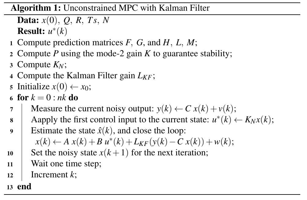
Example¶

Let's apply the unconstrained MPC regulator on an Unstable Non-minimum Phase system,

\begin{align*} Gp(s) = \dfrac{1-s}{(s-2)(s+1)} \end{align*}

in State-space form with the following conditions, \begin{align*} x(k+1) &= \begin{bmatrix} 1.1160 & 0.2110 \\ 0.1055 & 1.0100 \end{bmatrix} x(k)+ \begin{bmatrix} 0.1055\\ 0.0052 \end{bmatrix} u(k)+w(k)\\ y(k) &= \begin{bmatrix} -1 & 1 \end{bmatrix} x(k) + v(k)\\ x(0) & = [1.5 \quad 1]^\intercal\\ Ts &= 0.1, \quad N = 5, \quad k = 100\\ Q &= \begin{bmatrix} 1e2 & 0 \\ 0 & 1e2 \end{bmatrix} ,\quad R = 1\\ w(k) & \sim \mathcal{N}(0,1e^{-4}), \quad v(k) \sim \mathcal{N}(0,1e^{-4}) \end{align*}

Initial definitions¶

Global constants, the system, and the Penalty matrices. Mode-2 gain is used to calculate $P$.

Kalman Filter¶

Creating the Predicted Equality constraints $F$, and $G$¶

Creating the Predicted Cost matrices $H$, $L$, and $M$¶

Obtaining the Receding Horizon (RH) gain¶

For loop¶

Results¶

Input¶

The input control signal $u$ reaches zero relatively fast due the penalty cost $R=1$. Higher values of $R$ reaches zero slowly.

Output¶

The output $y$ converges around zero slowly due to $R$. Notice that the signal reflects the observation matrix $C=[-1~1]$.

States¶

The states start in the initial conditions $x(0)=[1.5~1]^\intercal$, and slowly converge to zero.

Phase-plot¶

The phase-plot shows more clearly the initial condition $x(0)$. Also, it shows the convergence around zero for $k \rightarrow \infty$

Cost value¶

The cost value $J^*_N(x(k),\mathbf{u}(k))$ indicates the descendent monotonic behaviour of the cost function $J_N(x(k),\mathbf{u}(k))$.

References¶

[1] James B. Rawlings and Mayne David Q. Model Predictive Control Theory and Design. Nob Hill Pub, Llc, 2009. ISBN: 9780975937709.

[2] Jan Maciejowski. Predictive Control with Constraints. Prentice Hall, 2000. ISBN: 978-0201398236.