Constrained MPC regulator with Kalman filter
Table of Contents
- 1 Constrained Model Predictive Control (MPC) regulator with Kalman filter
- 2 Pre-requisites
- 3 Background Theory
- 4 Constrained MPC
- 5 Problem Formulation
- 6 State constraints
- 7 Input constraints
- 8 Constructing the inequality constraints in compact form
- 9 QP solution
- 10 Stability
- 11 Algorithm
- 12 Example
- 13 Results
- 14 References
Constrained Model Predictive Control (MPC) regulator with Kalman filter
The following presents an unconstrained Linear Quadratic Model Predictive Control (LQ-MPC) simulation using Matlab-kernel for Jupyter Notebook. The code files can be used in Matlab natively.
Pre-requisites
- Knowledge in Control Systems theory.
- Convex quadratic optimization theory.
- Previous post of Unconstrained MPC.
- Jupyter Notebook with Matlab-kernel.
- Matlab.
- Install MPT3 tools for Matlab.
Background Theory
MPC is an optimization-based control strategy that solves a Finite-Horizon Linear Quadratic (FH-LQ) problem subject to constraints. A model of predicted states based on the system dynamics is used to minimize an objective function that satisfies constraints given the actual state. The obtained solution is a sequence of open-loop controls from which only the first one is implemented on the system, inducing feedback. The rest of the sequence is discarded and the process is repeated for the next sampling time, this method is often called Receding-Horizon (RH) principle. Advantages of MPC against other control strategies are the handling of constraints, and non-linearities.
Constrained MPC
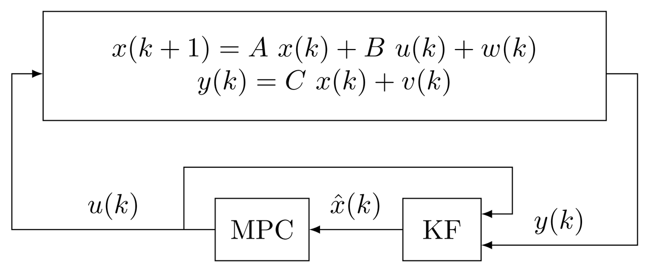
Consider the following discrete-time LTI state-space system \begin{equation*} \begin{aligned} x(k+1) &= A~x(k)+B~u(k)+w(k)\\ y(k) &= C~x(k)+v(k),\quad k=0,1,2,\dots \end{aligned} \end{equation*} where $x\in\mathbb{R}^n$, $u\in\mathbb{R}^m$, and $y\in\mathbb{R}^p$, are the states, input, and output vectors respectively. $A,~B,~C,$ are the state, input, and output matrices. $A,~B,~C$ are known, no uncertainties in the model, disturbances, and noise. $x(k)$ is available at each sampling time $k$. The process noise is $w(k)\sim \mathcal{N}(0,Q_w)$ with covariance $Q_w$, the measurement noise is $v(k)\sim \mathcal{N}(0,R_v)$ with covariance $R_v$, both are uncorrelated, and are in the form of Additive White Gaussian Noise (AWGN).
Problem Formulation
The objective is to regulate $x\rightarrow 0$ as $k\rightarrow \infty$ while minimizing the following cost function
\begin{align*}\tag{1} J_N(x(k),\mathbf{u}(k)) &= \sum_{j=0}^{N-1} \left( \|x(k+j|k)\|^2_Q + \|u(k+j|k)\|^2_R \right) + \|x(k+N|k)\|^2_P \\ &= \sum_{j=0}^{N-1} (x^\intercal(k+j|k)~Q~x(k+j|k)+ u^\intercal(k+j|k)~R~u(k+j|k) ) + x^\intercal(k+N|k)~P~x(k+N|k) \end{align*}
subject to,
\begin{align*}\tag{2} x(k+1+j|k) &= A~x(k+j|k)+B~u(k+j|k) \\ x(k|k) &= x(k) \\ P_x~x(k+j|k) &\leq q_x \\ P_u~u(k+j|k) &\leq q_u \\ P_{x_N}~x(k+N|k) &\leq q_{x_N} \end{align*}
for $ j=0,1,2,\dots,N-1$, where $Q\in\mathbb{R}^{n\times n}$ and $R\in\mathbb{R}^{m\times m}$ are the state penalty, and input penalty matrices. $P\in\mathbb{R}^{n\times n}$ is the terminal cost matrix, $N \in\mathbb{N}$ is the horizon length, $k$ is the sampling time, and $(k+j|k)$ can be defined as the next $(k+j)$ value given $k$. $P_x$, $P_u$, and $P_{x_N}$ are the states, input, and terminal state inequality constraints.
With the value function defined as \begin{align*} J^*_N(x(k),\mathbf{u}(k)) &= \min_{u(k)}~ J_N(x(k),\mathbf{u}(k)) \end{align*} the optimal control sequence is \begin{equation*} \begin{aligned} \mathbf{u}^*(k) &= \mathrm{arg}\min_{u(k)}~ J^*_N(x(k),\mathbf{u}(k))\\ &= \left\{ u^*(k|k),u^*(k+1|k),\dots,u^*(k+N-1|k) \right\} \end{aligned} \end{equation*}
State constraints
Let's define $P_x$ as box constraints \begin{align*} \underbrace{ \begin{bmatrix} +\textbf{I}_{n\times n}\\ -\textbf{I}_{n\times n} \end{bmatrix} }_{P_x} x(k+j|k) &\leq \underbrace{ \begin{bmatrix} +x_{max}\\ -x_{min} \end{bmatrix} }_{q_x} \end{align*}
formulate it with $P_{x_N}$ and $q_{x_N}$ (they will be defined in the stability section) \begin{align*} \begin{cases} P_x~x(k+j|k) &\leq q_x\\ P_{x_N}~x(k+N|k) &\leq q_{x_N} \end{cases} \end{align*} stacking, \begin{equation*} \begin{aligned} \underbrace{ \begin{bmatrix} P_x\\ 0\\ 0\\ \vdots\\ 0 \end{bmatrix} }_{\tilde{P_{x_0}}} x(k|k) + \underbrace{ \begin{bmatrix} 0 & 0 & \dots & 0 \\ P_x & 0 & \dots & 0 \\ 0 & P_x & \dots & 0 \\ \vdots & \vdots & \ddots & \vdots \\ 0 & 0 & \dots & P_{x_N} \end{bmatrix} }_{\tilde{P_x}} \underbrace{ \begin{bmatrix} x(k+1|k)\\ x(k+2|k)\\ \vdots\\ x(k+N|k) \end{bmatrix} }_{\mathbf{x}(k)} \leq \underbrace{ \begin{bmatrix} q_x\\ q_x\\ q_x\\ \vdots\\ q_{x_N} \end{bmatrix} }_{\tilde{q_x}} \end{aligned} \end{equation*} results in \begin{align}\tag{3} \tilde{P_x}~\mathbf{x}(k)\leq \tilde{q_x}-\tilde{P}_{x_0}~x(k) \end{align}
Input constraints
Let's define $P_u$ as box constraints \begin{align*} \underbrace{ \begin{bmatrix} +\textbf{I}_{m\times m}\\ -\textbf{I}_{m\times m} \end{bmatrix} }_{P_u} u(k+j|k) &\leq \underbrace{ \begin{bmatrix} +u_{max}\\ -u_{min} \end{bmatrix} }_{q_x} \end{align*}
then, \begin{align*} P_u~u(k+j|k)\leq q_u \end{align*} stacking, \begin{equation*} \begin{aligned} \underbrace{ \begin{bmatrix} P_u & 0 & \dots & 0\\ 0 & P_u & \dots & 0\\ \vdots & \vdots & \ddots & \vdots\\ 0 & 0 & \dots & P_u \end{bmatrix} }_{\tilde{P_u}} \underbrace{ \begin{bmatrix} u(k|k)\\ u(k+1|k)\\ \vdots\\ u(k+N-1|k) \end{bmatrix} }_{\mathbf{u}(k)} \leq \underbrace{ \begin{bmatrix} q_u\\ q_u\\ \vdots\\ q_u \end{bmatrix} }_{\tilde{q_u}} \end{aligned} \end{equation*} results in \begin{align}\tag{4} \tilde{P_u}~\mathbf{u}(k)\leq \tilde{q_u} \end{align}
Constructing the inequality constraints in compact form
If Constructing inequality constraints in a compact form \begin{align*} \begin{cases} \tilde{P_u}~\mathbf{u}(k) &\leq \tilde{q_u}\\ \tilde{P_x}~\mathbf{x}(k) &\leq \tilde{q_x}-\tilde{P}_{x_0}~x(k) \end{cases} \end{align*} using the predicted equality constraints $\mathbf{x}(k)=F~x(k)+G~\mathbf{u}(k)$ (rev previous post of Unconstrained MPC) \begin{align*} \tilde{P_x}(F~x(k)+G~\mathbf{u}(k)) &\leq \tilde{q_x}-\tilde{P}_{x_0}~x(k)\\ \tilde{P_x}~G~\mathbf{u}(k) &\leq \tilde{q_x}+(-\tilde{P}_{x_0}-\tilde{P_x}~F)~x(k) \end{align*} stacking \begin{equation*} \begin{aligned} \underbrace{ \begin{bmatrix} \tilde{P_u}\\ \tilde{P_x}~G \end{bmatrix} }_{P_c} \mathbf{u}(k) \leq \underbrace{ \begin{bmatrix} \tilde{q_u}\\ \tilde{q_x} \end{bmatrix} }_{q_c} + \underbrace{ \begin{bmatrix} 0\\ -\tilde{P}_{x_0}-\tilde{P_x}~F \end{bmatrix} }_{S_c} x(k) \end{aligned} \end{equation*} therefore, \begin{align}\tag{5} P_c~\mathbf{u}(k) \leq q_c+S_c~x(k) \end{align}
QP solution
The LQ-MPC problem in constrained compact form is to minimize \begin{align}\tag{6} J^*_N(x(k),\mathbf{u}(k)) &= \min_{\mathbf{u}(k)}~\frac{1}{2} \mathbf{u}(k)^\intercal~H~\mathbf{u}(k)+c^\intercal~\mathbf{u}(k)+\alpha \end{align} subject to, \begin{align*} P_c~\mathbf{u}(k) &\leq q_c+S_c~x(k) \end{align*} where the optimal solution can be defined as
\begin{align*} \mathbf{u}^*(k) &= \mathrm{arg}\min_{u(k)}~ \left. \begin{cases} \dfrac{1}{2} \mathbf{u}(k)^\intercal H \mathbf{u}(k)+x^\intercal(k) L^\intercal \mathbf{u}(k)+\alpha~: P_c \mathbf{u} \leq q_c+S_c x(k) \end{cases} \right\} \\ &= \left\{ u^*(k|k),u^*(k+1|k),\dots,u^*(k+N-1|k) \right\} \end{align*}
with the same definitions of $H,~L$ and $\alpha$ of the unconstrained MPC case.
Applying the RH principle leads to the implicit nonlinear time-variant control law, \begin{align}\tag{7} u^*(k|k) = \kappa_N \left( x(k) \right) \end{align} and it is defined for $x(k)\in \mathcal{X}_N$, where $\mathcal{X}_N$ is the feasibility region.
The feasibility region $\mathcal{X}_N$ is the set of states for which the cost function has a solution, and is defined as \begin{align*} \mathcal{X}_N = \{x(k):\mathcal{U}_N(x(k)) \neq 0\} \end{align*} where the feasible set $\mathcal{U}_N$ is \begin{align*} \mathcal{U}_N(x(k)) &= \{ \mathbf{u}(k) : P_c~\mathbf{u}(k) \leq q_c+S_c~x(k) \} \end{align*} Also, the input constraint set is \begin{align*} \mathcal{U} &=\{ u(k) : P_u~u(k)\leq q_u \} \subseteq \mathbb{R}^m\\ \end{align*} the state constraint set is \begin{align*} \mathcal{X} &=\{ x(k) : P_x~x(k)\leq q_x \} \subseteq \mathbb{R}^n\\ \end{align*} and the terminal constraint set is \begin{align*} \mathcal{X}_f &=\{ x(k) : P_{x_N}~x(k)\leq q_{x_N} \} \subseteq \mathbb{R}^n \end{align*}
Stability
To guarantee stability, the aim is to construct a terminal constraint set $\mathcal{X}_f$ such that feasibility of the problem for $x(k)$ satisfies constraints for mode-2, \begin{equation*} \begin{aligned} x(k+N+j|k) &\in \mathcal{X},~j=1,2,...\\ u(k+N+j|k) &\in \mathcal{U},~j=1,2,... \end{aligned} \end{equation*}
An approach is to use deadbeat mode-2 constraints as terminal constraints. For $j=N,\dots,N+n-1$ in \begin{equation*} \begin{aligned} x(k+j|k) &= (A+B~K)^j~x(k+N|k)\\ u(k+j|k) &= K(A+B~K)^j~x(k+N|k) \end{aligned} \end{equation*} that is, extending the constraints for $n$ steps beyond mode-1, \begin{equation*} \begin{aligned} \underbrace{ \overbrace{ \begin{bmatrix} Px & 0 & \dots & 0 \\ P_u K & 0 & \dots & 0 \\ 0 & P_x & \dots & 0 \\ 0 & P_u K & \dots & 0 \\ \dots & \dots & \dots & \dots \end{bmatrix} }^{\mathcal{M}} \begin{bmatrix} (A+B K)^0\\ (A+B K)^1 \\ \vdots\\ (A+B K)^{n-1} \end{bmatrix} }_{P_{x_N}} x(k+N|k) \leq \underbrace{ \begin{bmatrix} q_x\\ q_u\\ q_x\\ q_u\\ \vdots \end{bmatrix} }_{q_{x_N}} \end{aligned} \end{equation*} where \begin{equation*} \begin{aligned} \mathcal{M} = \textbf{I}_{n\times n} \otimes \begin{bmatrix} P_x\\ P_u K \end{bmatrix} ,\qquad q_{x_N} = \textbf{1}_{n\times 1} \otimes \begin{bmatrix} q_x\\ q_u \end{bmatrix} \end{aligned} \end{equation*} Therefore, for any $x(k+N|k) \in \mathcal{X}_f$ \begin{align}\tag{8} \mathcal{X}_f = \{ x(k+N|k) \in \mathbb{R}^n : P_{x_N}~x(k+N|k) \leq q_{x_N} \} \end{align}
This terminal constraint set has the property to be an admissible invariant set, which means that mode-2 constraints are satisfied, and mode-2 predictions stay within $\mathcal{X}_f$. This concept is called admissibility implies stability, in other words \begin{align*} x(k+N|k) \in \mathcal{X}_f &\Rightarrow x(k+N|k) \in \mathcal{X}\\ u(k+N|k) &= K~(x(k+N|k)) \in \mathcal{U} \end{align*}
In conclusion, the stability is guaranteed for the following conditions,
- $(A,B)$ is stabilizable.
- $Q\succeq 0,~R\succ 0$
- $(Q^{1/2},A)$ is observable.
- $P$ satisfies the Lyapunov equation for some stabilizing $K$, $(A+B~K)^\intercal~P~(A+B~K)-P=-(Q+K^\intercal~R~K)$
- $\mathcal{X}_f$ is an admissible invariant set for mode-2 dynamics: $x(k+1)=(A+B~K)~x(k)$
then, given an $x(k)\in \mathcal{X}_N$,
- $J^*_N(x(k))$ is a Lyapunov function for mode-1 dynamics: $x(k+1)=Ax(k)+B\kappa_N(x(k))$, and recursively feasible, that is: if there is a feasible solution $J^*_N(x(k))$, then all subsequent solutions ${J^*_N(x(k+1)),~J^*_N(x(k+2)),\dots}$ exist and are feasible within $\mathcal{X}_N$.
- All constraints are satisfied.
- The origin $x=0$ is asymptotically stable with Region of Attraction (RoA) $\mathcal{X}_N$.
- $\mathcal{X}_N$ is an admissible invariant set for mode-1 dynamics:$x(k+1)=Ax(k)+B\kappa_N(x(k))$.
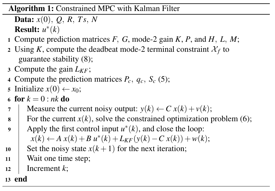
Algorithm
Example
Let's apply the constrained MPC regulator on an Unstable Non-minimum Phase system
\begin{align*} Gp(s) = \dfrac{1-s}{(s-2)(s+1)} \end{align*}
in State-space form with the following conditions \begin{align*} x(k+1) &= \begin{bmatrix} 1.1160 & 0.2110 \\ 0.1055 & 1.0100 \end{bmatrix} x(k)+ \begin{bmatrix} 0.1055\\ 0.0052 \end{bmatrix} u(k)+w(k)\\ y(k) &= \begin{bmatrix} -1 & 1 \end{bmatrix} x(k) + v(k)\\ x(0) & = [1.5 \quad 1]^\intercal\\ Ts &= 0.1, \quad N = 5, \quad k = 100\\ Q &= \begin{bmatrix} 1e2 & 0 \\ 0 & 1e2 \end{bmatrix} ,\quad R = 1\\ w(k) & \sim \mathcal{N}(0,1e^{-4}), \quad v(k) \sim \mathcal{N}(0,1e^{-4}) \end{align*}
Constraints \begin{align*} |x| \leq 2, \quad |u| \leq 7 \end{align*}
Init
% Global constants
clear variables;
options = optimoptions(@quadprog,'MaxIterations',1000,'ConstraintTolerance',1e-12,'Display','off');

x0 = [1.5; 1];  % initial conditions
nk = 100;       % simulation steps
Ts = 0.1;       % sampling time
t = Ts*(0:nk);  % simulation time
N = 5;          % horizon

% System
% sys = (-s+1)/((s-2)*(s+1));
[Ac,Bc,Cc,Dc] = tf2ss([-1 1],[1 -1 -2]);
Bdc = [1;0]; Ddc = 0;
sysc = ss(Ac,[Bc Bdc],Cc,[Dc Ddc]);

sysd = c2d(sysc,Ts);
A = sysd.A;
B = sysd.B(:,1);
Bd = sysd.B(:,2);
C = sysd.C;
D = sysd.D(:,1);

% Penalty Cost matrices
Q = [ 1e2   0
      0   1e2];
R = 1;

% Mode-2 gain
K = -dlqr(A,B,Q,R)

% Terminal Cost matrix
Phi = A+B*K;
S = Q+K'*R*K;
P = dlyap(Phi',S)

% System Dimensions
n  = size(A, 1);    % Number of State variables
m  = size(B, 2);    % Number of Input variables
p  = size(C, 1);    % Number of Output measurments
Kalman Filter
% Stream of process noise and measurement noise (AWGN)
rng default;                % For reproducibility (seed)
mu_Qw = [0, 0];             % mean of the states (mu_x1, mu_x2)
Qw = diag([1e-4, 1e-4]);    % process noise covariance. Qw=diag[sigma_x1^2, sigma_x2^2]
w = mvnrnd(mu_Qw,Qw,nk+1);  % noise input vector
% cov(w)                    % covariance matrix of w
% scatter(w(:,1),w(:,2))

mu_Rv = 0;                  % mean of the measurements
Rv = (1e-4)*eye(1);         % measurement noise covariance. Rv=sigma^2
v = mvnrnd(mu_Rv,Rv,nk+1);  % noise output vector

% KF Steady-State
[kest,LKF,Ps] = kalman(sysd,Qw,Rv);
LKF
Constraints
% Input constraints
u_max = 7; u_min = 7;
Pu = [1; -1];
qu = [u_max; u_min];
U = Polyhedron(Pu,qu);
% U.plot('alpha',0.1,'LineStyle','--');

% State constraints
x_max = 2; x_min = 2;
Px = [eye(n); -eye(n)];
qx = [ones(n,1)*x_max; ones(n,1)*x_min];
X = Polyhedron(Px,qx);
% X.plot('alpha',0.0,'LineStyle','--');
Deadbeat Terminal Inequality State constraints
K = -dlqr(A,B,Q,R);
nn = N;
Maux = [];
for i=0:nn-1
    Maux = [Maux;(A+B*K)^(i)];
end
Mm = kron(eye(nn),[Px; Pu*K]);

% regulation
PxN = Mm*Maux;
qxN = kron(ones(nn,1),[qx; qu]);% deadbeat terminal inequality constraints
Xf = Polyhedron(PxN,qxN);
MPT3 - Control Invariant Set (CIS)
% computes a control invariant set for LTI system x^+ = A*x+B*u
% When applied to an autonomous system , the method computes the maximal positively invariant set.
% When applied to a non-autonomous system, the maximal control invariant set is computed.
system = LTISystem('A', A, 'B', B);
system.x.min = [-x_min; -x_min];
system.x.max = [x_max; x_max];
system.u.min = -u_min;
system.u.max = u_max;
InvSet = system.invariantSet(); % XN = Control Invariant Set
Pxx = InvSet.A; qxx = InvSet.b;
% InvSet.plot('alpha',0.1,'color','lightblue')
XN = Polyhedron(InvSet.A,InvSet.b);
% figure,XN.plot('alpha',0.1,'color','red');
Prediction, Constraint and Cost matrices
Predictions matrices function $F$ and $G$
%%file 'C:/Users/zurit/OneDrive/blog/files/MPCc/predict_mats.m'

function [F,G] = predict_mats(A,B,N)
    % P. Trodden, 2015.

    % dimensions
    n = size(A,1);
    m = size(B,2);

    % allocate
    F = zeros(n*N,n);
    G = zeros(n*N,m*(N-1));

    % form row by row
    for i = 1:N
        %  F
        F(n*(i-1)+(1:n),:) = A^i;

        % G
        % form element by element
        for j = 1:i
            G(n*(i-1)+(1:n),m*(j-1)+(1:m)) = A^(i-j)*B;
        end
    end
end
cd 'C:/Users/zurit/OneDrive/blog/files/MPCc'
% Prediction matrices
[F,G] = predict_mats(A,B,N);
Constraints matrices $P_c$, $q_c$, and $S_c$
%%file 'C:/Users/zurit/OneDrive/blog/files/MPCc/constraint_mats.m'

function [Pc, qc, Sc, Pu_tilde, Px_tilde, qx_tilde, Px0_tilde] = constraint_mats(F,G,Pu,qu,Px,qx,Pxf,qxf)
    % P. Trodden, 2017.

    % input dimension
    m = size(Pu,2);

    % state dimension
    n = size(F,2);

    % horizon length
    N = size(F,1)/n;

    % number of input constraints
    ncu = numel(qu);

    % number of state constraints
    ncx = numel(qx);

    % number of terminal constraints
    ncf = numel(qxf);

    % if state constraints exist, but terminal ones do not, then extend the
    % former to the latter
    if ncf == 0 && ncx > 0
        Pxf = Px;
        qxf = qx;
        ncf = ncx;
    end

    %% Input constraints

    % Build "tilde" (stacked) matrices for constraints over horizon
    Pu_tilde = kron(eye(N),Pu);
    qu_tilde = kron(ones(N,1),qu);
    Scu = zeros(ncu*N,n);

    %% State constraints

    % Build "tilde" (stacked) matrices for constraints over horizon
    Px0_tilde = [Px; zeros(ncx*(N-1) + ncf,n)];
    if ncx > 0
        Px_tilde = [kron(eye(N-1),Px) zeros(ncx*(N-1),n)];
    else
        Px_tilde = zeros(ncx,n*N);
    end
    Pxf_tilde = [zeros(ncf,n*(N-1)) Pxf];
    Px_tilde = [zeros(ncx,n*N); Px_tilde; Pxf_tilde];
    qx_tilde = [kron(ones(N,1),qx); qxf];

    %% Final stack
    if isempty(Px_tilde)
        Pc = Pu_tilde;
        qc = qu_tilde;
        Sc = Scu;
    else
        % eliminate x for final form
        Pc = [Pu_tilde; Px_tilde*G];
        qc = [qu_tilde; qx_tilde];
        Sc = [Scu; -Px0_tilde - Px_tilde*F];
    end
end
cd 'C:/Users/zurit/OneDrive/blog/files/MPCc'
% Constraint matrices
[Pc,qc,Sc,Pu_tilde,Px_tilde,qx_tilde,Px0_tilde] = constraint_mats(F,G,Pu,qu,Px,qx,PxN,qxN);
Cost matrices function $H$, $L$, and $M$
%%file 'C:/Users/zurit/OneDrive/blog/files/MPCc/cost_mats.m'

function [H,L,M] = cost_mats(F,G,Q,R,P)
    % P. Trodden, 2015.

    % get dimensions
    n = size(F,2);
    N = size(F,1)/n;

    % diagonalize Q and R
    Qd = kron(eye(N-1),Q);
    Qd = blkdiag(Qd,P);
    Rd = kron(eye(N),R);

    % Hessian
    H = 2*G'*Qd*G + 2*Rd;

    % Linear term
    L = 2*G'*Qd*F;

    % Constant term
    M = F'*Qd*F + Q;

    % make sure the Hessian is symmetric
    H=(H+H')/2;
end
cd 'C:/Users/zurit/OneDrive/blog/files/MPCc'
% Cost matrices
[H,L,M] = cost_mats(F,G,Q,R,P)
Unconstrained MPC
%% Unconstrained MPC: RH-FH-LQR/LQ-MPC
Ku = -H\L;     % optimized solution
KN = Ku(1,:); % RH-FH gain, first row of the m-row matrix
For loop
cd 'C:/Users/zurit/OneDrive/blog/files/MPCc'

% MPC unconstrained
x_mpc_u = x0;
xs_mpc_u = zeros(n,nk+1);
us_mpc_u = zeros(m,nk+1);


% MPC constrained
x_mpc = x0;
xs_mpc = zeros(n,nk+1);
us_mpc = zeros(m,nk+1);

for k = 1:nk+1

    % --- Perturbation -----------------------------------------------
        if k>=40 && k<=50
            d = -3.8;
        else
            d=0;
        end


    %% --- MPC unconstrained --------------------------------------------------------------
    xs_mpc_u(:,k) = x_mpc_u;
    y_mpc_u(k) = C*x_mpc_u+v(k);
    us_mpc_u(:,k) = KN*x_mpc_u;
    x_mpc_u = A*x_mpc_u+B*us_mpc_u(:,k) + LKF*(y_mpc_u(k)-C*x_mpc_u)+w(k,:)'+Bd*d;
    J_mpc_u(k) = x_mpc_u'*Q*x_mpc_u+us_mpc_u(:,k)'*R*us_mpc_u(:,k);

    %% --- MPC constrained -------------------------------------------------------------
    xs_mpc(:,k) = x_mpc;
    y_mpc(k) = C*x_mpc+v(k);
    % Constrained MPC control law (RH-FH) LQ-MPC at every step k
    [Ustar,~,flag] = quadprog(H,L*x_mpc,Pc,qc+Sc*x_mpc,[],[],[],[],[],options);

    % check feasibility
    if flag < 1
        disp(['MPC Optimization is infeasible at k = ',num2str(k)]);
        break;
    end
    % Store input
    us_mpc(:,k) = Ustar(1);
    % Feedback x(k+1)=A*x(k)+B*u(k)
    x_mpc = A*x_mpc+B*us_mpc(:,k) + LKF*( y_mpc(k)-C*x_mpc )+w(k,:)'+Bd*d;
    % Cost Value
    J_mpc(k) = 0.5*Ustar(1:N,:)'*H*Ustar(1:N,:)+xs_mpc(:,k)'*L'*Ustar(1:N,:)+...
                  xs_mpc(:,k)'*M*xs_mpc(:,k);

end
Results
For comparision, let's simulate Constrained MPC and Unconstrained MPC
- MPCc = Constrained MPCc
- MPCu = Unconstrained MPC
MPCu + MPCc: input and output
figure;
    % Input
    subplot(2,1,1);
    hold on;
    stairs(t,us_mpc_u,'--','LineWidth',1);
    stairs(t,us_mpc,'-.','LineWidth',1);
    ylabel('$u$','Interpreter','Latex');
    legend('MPCu','MPCc',...
            'Location','southeast',...
            'Interpreter','Latex');
    grid on;

    % Output
    subplot(2,1,2);
    hold on;
    plot(t,y_mpc_u,'--','LineWidth',1);
    plot(t,y_mpc,'-.','LineWidth',1);
    ylabel('$y$','Interpreter','Latex');
    legend('MPCu','MPCc',...
           'Location','northeast',...
           'Interpreter','Latex');
    grid on;

MPCu + MPCc: states and phase plot
figure;
    % States
    subplot(2,1,1);
    hold on;
    plot(t,xs_mpc_u(1,:),'--',t,xs_mpc_u(2,:),'--','LineWidth',1);
    plot(t,xs_mpc(1,:),'-.',t,xs_mpc(2,:),'-.','LineWidth',1);
    xlabel('Time step [s]');
    ylabel('$x_1,~x_2$','Interpreter','Latex','Fontsize',12);
    legend('$x_1~$ MPCu','$x_2~$ MPCu',...
           '$x_1~$ MPCc','$x_2~$ MPCc',...
            'Location','bestoutside',...
            'Interpreter','Latex');
    grid on;

    % Phase-plot + terminal set Xf
    subplot(2,1,2);
    hold on;
    plot(xs_mpc_u(1,:),xs_mpc_u(2,:),'--x','LineWidth',1);
    plot(xs_mpc(1,:),xs_mpc(2,:),'--o','LineWidth',1);
    X.plot('alpha',0.0,'LineStyle','--');
    InvSet.plot('alpha',0.1,'color','lightblue');
    Xf.plot('alpha',0.1,'color','green','LineStyle','-.');
    xlabel('$x_1$','Interpreter','Latex');
    ylabel('$x_2$','Interpreter','Latex');
%     title('Phase-plot');
    legend('MPCu','MPCc',...
           '$X$','$X_N$','$X_f$',...
           'Location','bestoutside',...
           'Interpreter','Latex');
    grid on;

MPCu + MPCc: Cost value
figure;
    hold on;
    plot(t,J_mpc_u,'--','LineWidth',1);
    plot(t,J_mpc,'--','LineWidth',1);
    xlabel('Time step [s]');
    ylabel('$J(k)$','Interpreter','Latex','Fontsize',12);
    legend('MPCu','MPCc',...
            'Location','southeast',...
            'Interpreter','Latex');
    grid on;

References
[1] James B. Rawlings and Mayne David Q. Model Predictive Control Theory and Design. Nob Hill Pub, Llc, 2009. ISBN: 9780975937709.
[2] Jan Maciejowski. Predictive Control with Constraints. Prentice Hall, 2000. ISBN: 978-0201398236.
Comments
Comments powered by Disqus