Dynamic model of a DC motor with gear train

Table of Contents

Source code

Version PDF/HTML. LaTex source code on GitHub.

Introduction

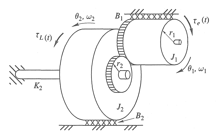
The objective is to model the dynamics of a DC servo motor with gear train, Fig. 1, and to deduce two equilibrium points.

DCmotor
Fig.1 - DC servo motor with gear train.

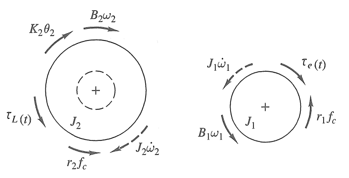
Free-body diagram analysis

The system can be decomposed in two sections: a rotational mechanical, and an electro-mechanical. The rotational mechanical can be derived as follows,

Rotational_free-body
Fig.2 - Rotational mechanical free-body diagram.

where $\theta$ is the angular displacement, $\omega$ is the angular speed, $B$ is the rotational viscous-damping coefficient, $K$ is the stiffness coefficient, $J$ is the moment of inertia, $f_c$ is the contact force between two gears, and $r$ is the gear radius.

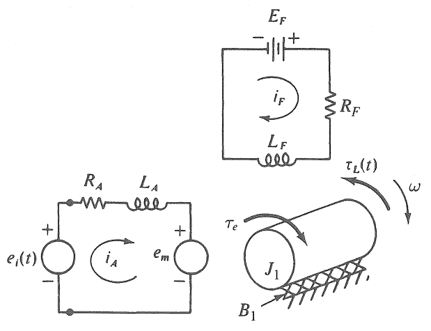
The electromechanical section (DC motor) is

Electromechanical_free-body
Fig.3 - Electro-mechanical free-body diagram.

where $R_F$ is the field resistance, $L_F$ is the field inductance, $E_F$ is the applied constant field voltage, and $i_F$ is the input field current. $R_A$ is the stationary resistance, $L_A$ is the stationary inductance, and $e_m$ is the induced voltage, $i_A$ is the input stationary current, and $e_i(t)$ is the applied armature voltage, and $\tau_e$ is the electro-mechanical driving torque exerted on the rotor.

If the flux density $\mathcal{B}$ is

\begin{align} \mathcal{B} & = \frac{\phi(i_F)}{A} \end{align}

the torque on the rotor is

s \begin{align} \tau_e & = \mathcal{B} l a~i_A \nonumber \\ \tau_e & = \frac{l a}{A} \phi(i_F) i_A \label{eq:tau_e} \end{align}

where $\phi(i_F)$ is the flux induced by $i_F$, $A$ is the cross-sectional area of the flux path in the air gap between the rotor and stator, $l$ is the total length of the armature conductors within the magnetic field, and $a$ is the radius of the armature.

Also, the voltage induced in the armature $e_m$ can be written as

\begin{align} e_m & = \frac{l a}{A} \phi(i_F) \omega \end{align}

where both, $\tau_e$ and $e_m$, depend on the geometry of the DC motor.

Dynamic system

We begin applying D'Alembert's law (restatement of Newton's law) to the rotational mechanical section.

\begin{align} \sum \tau_{all} & = 0 \nonumber \\ J_1 \dot{\omega}_1 + B_1 \omega_1 + r_1 f_c & = \tau_e(t) \label{eq:Rot1} \\ J_2 \dot{\omega}_2 + B_2 \omega_2 + K_2 \theta - r_2 f_c & = \tau_L(t) \label{eq:Rot2} \end{align}

where $\tau_{all}$ are the torques acting on a body, $K\theta$ is the stiffness torque, $B\omega$ is the viscous-frictional torque, $J\dot{\omega}$ is the inertial torque, $\tau_e(t)$ is the driving torque, $\tau_L(t)$ is the load torque, and $r f_c$ is the contact torque.

Due to the relation between gears,

\begin{align*} \theta_1 & = N \theta_2 \\ \omega_1 & = N \omega_2 \\ \dot{\omega}_1 & = N \dot{\omega}_2 \\ N & = \frac{r_2}{r_1} \end{align*}

where $N$ is the gear radius relation. We solve \eqref{eq:Rot1} and \eqref{eq:Rot2} in terms of $\omega_2$ and $\theta_2$,

\begin{align} (J_2+N^2 J_1)\dot{\omega}_2+(B_2+N^2 B_1)\omega_1+K_2 \theta_2-N \tau_e(t)-\tau_L(t) = 0 \nonumber \end{align}

defining the relations

\begin{align*} J_{eq} & = J_2+N^2 J_1 \\ B_{eq} & = B_2+N^2 B_1 \end{align*}

it becomes in

\begin{align} J_{eq} \dot{\omega}_2+B_{eq} \omega_2+K_2 \theta_2-N \tau_e(t)-\tau_L(t) = 0 \label{eq:Rot3} \end{align}

Now, let us derive the equations of the electro-mechanical section using Kirchoff's law.

\begin{align} \sum V_{all} & = 0 \nonumber \\ e_m+V_{L_{A}}+V_{R_{A}} & = e_i(t) \label{eq:Elec1} \end{align}

where $V_{all}$ are the induced voltages on the rotor and stator, $V_{L_{A}}$ is the stationary resistance voltage, $V_{R_{A}}$ is the stationary inductance voltage.

If $i_F$ is defined as constant, then \eqref{eq:tau_e} is

\begin{align} \tau_e(t) & = \left( \frac{l a}{A} \phi(i_F) \right) i_A(t) \nonumber \\ \tau_e(t) & = \alpha i_A(t) \end{align}

where $\alpha$ is the internal parameters of the DC motor.

Then, simplifying and using \eqref{eq:Rot3} and \eqref{eq:Elec1} the dynamic system is,

\begin{align} J_{eq} \dot{\omega}_2+B_{eq} \omega_2+K_2 \theta_2-N \tau_e - \tau_L & = 0 \\ L_A \dot{i}_A + R_A i_A + \alpha \omega_1 - e_i & = 0 \end{align}

State-space equations

Let us define the state-space equations for $x=\left[ \theta_2~\dot{\theta}_2~i_A \right]^{\intercal}$. From the dynamic system,

\begin{align*} J_{eq} \ddot{\theta}_2+B_{eq} \dot{\theta}_2+K_2 \theta_2-N \alpha i_A-\tau_L & = 0 \\ L_A \dot{i}_A + R_A i_A + \alpha \omega_1 - e_i & = 0 \end{align*}

reordering,

\begin{align*} \ddot{\theta}_2 & = -\frac{B_{eq}}{J_{eq}} \dot{\theta}_2 - \frac{K_2}{J_{eq}} \theta_2 + \frac{N \alpha}{J_{eq}} i_A - \frac{1}{J_{eq}} \tau_L \\\ \dot{i}_A & = -\frac{R_A}{L_A} i_A -\frac{N \alpha}{L_A} \dot{\theta}_2 + \frac{1}{L_A} e_i \end{align*}

defining the states as

\begin{align*} \begin{cases} x_1 & = \theta_2, \quad \dot{x}_1 = \dot{\theta}_2 = x_2 \\\ x_2 & = \dot{\theta}_2, \quad \dot{x}_2 = \ddot{\theta}_2 = -\frac{B_{eq}}{J_{eq}} x_2 - \frac{K_2}{J_{eq}} x_1 + \frac{N \alpha}{J_{eq}} x_3 - \frac{1}{J_{eq}} \tau_L \\\ x_3 & = i_A, \quad \dot{x}_3 = \dot{i}_A = -\frac{R_A}{L_A} x_3 -\frac{N \alpha}{L_A} x_2 + \frac{1}{L_A} e_i \end{cases} \end{align*}

then

\begin{align} \begin{bmatrix} \dot{x}_1 \\ \dot{x}_2 \\ \dot{x}_3 \end{bmatrix} &= \underbrace{ \begin{bmatrix} 0 & 1 & 0 \\ -\frac{K_2}{J_{eq}} & -\frac{B_{eq}}{J_{eq}} & \frac{N \alpha}{J_{eq}} \\ 0 & -\frac{N \alpha}{L_A} & -\frac{R_A}{L_A} \end{bmatrix} }_A \underbrace{ \begin{bmatrix} x_1 \\ x_2 \\ x_3 \end{bmatrix} }_\mathbf{x} + \underbrace{ \begin{bmatrix} 0 & 0 & 0 \\ 0 & -\frac{1}{J_eq} & 0 \\ 0 & 0 & \frac{1}{L_A} \end{bmatrix} }_B \underbrace{ \begin{bmatrix} 0 \\ \tau_L \\ e_i \end{bmatrix} }_\mathbf{u} \\ \mathbf{\dot{x}} &= A \mathbf{x} + B \mathbf{u} \label{eq:sys1} \end{align}

The output $y=\dot{\omega}_2$ can be defined as

\begin{align} y &= \underbrace{ \begin{bmatrix} 0 & 1 & 0 \end{bmatrix} }_C \begin{bmatrix} x_1 \\ x_2 \\ x_3 \end{bmatrix} + \underbrace{ \begin{bmatrix} 0 & 0 & 0 \end{bmatrix} }_D e_i \\ y &= C \mathbf{\dot{x}} \end{align}

Equilibrium point $\mathbf{x_0}$

Using $\mathbf{\dot{x}}=0$ in \eqref{eq:sys1}, the equilibrium point $\mathbf{x_0}$ can be calculated as

\begin{align} 0 & = A \mathbf{x_0} +B \mathbf{u} \\ \mathbf{x_0} & = - A^{-1} B \mathbf{u} \\ \begin{bmatrix} x_{1_0} \\ x_{2_0} \\ x_{3_0} \end{bmatrix} & = - \begin{bmatrix} 0 & 1 & 0 \\ -\frac{K_2}{J_{eq}} & -\frac{B_{eq}}{J_{eq}} & \frac{N \alpha}{J_{eq}} \\ 0 & -\frac{N \alpha}{L_A} & -\frac{R_A}{L_A} \end{bmatrix}^{-1} \begin{bmatrix} 0 & 0 & 0 \\ 0 & -\frac{1}{J_eq} & 0 \\ 0 & 0 & \frac{1}{L_A} \end{bmatrix} \begin{bmatrix} 0 \\ \tau_L \\ e_i \end{bmatrix} \end{align}

Solving for no external torque $\tau_L=0$, constant applied armature voltage $e_i=E_0$, and $K_2 \neq 0$,

\begin{align*} 0 & = x_{2_0} \\ 0 & = -\frac{K_2}{J_{eq}} x_{1_0} -\frac{B_{eq}}{J_{eq}} x_{2_0} + \frac{N \alpha}{J_{eq}} x_{3_0} \\ 0 & = -\frac{N \alpha}{L_A} x_{2_0} -\frac{R_A}{L_A} x_{3_0} + \frac{1}{L_A} E_0 \end{align*}

due to $x_{2_0}=0$, we have

\begin{align*} 0 & = -\frac{K_2}{J_{eq}} x_{1_0} + \frac{N \alpha}{J_{eq}} x_{3_0} \\ 0 & = -\frac{R_A}{L_A} x_{3_0} + \frac{1}{L_A} E_0 \end{align*} then \begin{align*} x_{1_0} & = \frac{N \alpha}{K_2 R_A} E_0 \\ x_{3_0} & = \frac{1}{R_A} E_0 \end{align*} therefore the equilibrium point is \begin{align} \mathbf{x_0} &= \begin{bmatrix} x_{1_0} \\ x_{2_0} \\ x_{3_0} \end{bmatrix} = \begin{bmatrix} \frac{N \alpha}{K_2 R_A} \\ 0 \\ \frac{1}{R_A} \end{bmatrix} E_0 \end{align}

This equilibrium point indicates that a $\textbf{constant angular displacement (twist)}$ produced by $x_{1_0}=\theta_{2_0}$ is sufficient to balance the constant applied armature voltage $e_i=E_0$.

On the other hand, if we solve for no external torque $\tau_L=0$, constant applied armature voltage $e_i=E_0$, and no stiffness $K_2 = 0$. The problem is,

\begin{align*} \begin{bmatrix} x_{1_0} \\ x_{2_0} \\ x_{3_0} \end{bmatrix} & = - \begin{bmatrix} 0 & 1 & 0 \\ 0 & -\frac{B_{eq}}{J_{eq}} & \frac{N \alpha}{J_{eq}} \\ 0 & -\frac{N \alpha}{L_A} & -\frac{R_A}{L_A} \end{bmatrix}^{-1} \begin{bmatrix} 0 & 0 & 0 \\ 0 & -\frac{1}{J_eq} & 0 \\ 0 & 0 & \frac{1}{L_A} \end{bmatrix} \begin{bmatrix} 0 \\ 0 \\ E_0 \end{bmatrix} \end{align*}

if we eliminate $x_{1_0}$ because the first column of $A^{-1}$ has zeros, the problem reduces to

\begin{align} \begin{bmatrix} x_{2_0} \\ x_{3_0} \end{bmatrix} & = - \begin{bmatrix} -\frac{B_{eq}}{J_{eq}} & \frac{N \alpha}{J_{eq}} \\ -\frac{N \alpha}{L_A} & -\frac{R_A}{L_A} \end{bmatrix}^{-1} \begin{bmatrix} -\frac{1}{J_eq} & 0 \\ 0 & \frac{1}{L_A} \end{bmatrix} \begin{bmatrix} 0 \\ E_0 \end{bmatrix} \end{align}

solving, we have

\begin{align} \begin{bmatrix} x_{2_0} \\ x_{3_0} \end{bmatrix} & = \begin{bmatrix} \frac{N \alpha}{B_{eq} R_A+(N \alpha)^2}\\ \frac{-B_{eq}}{B_{eq} R_A+(N \alpha)^2} \end{bmatrix} E_0 \end{align}

which indicates that a $\textbf{constant angular speed}$ produced by $x_{2_0}=\dot{\theta_{2_0}}$ is needed to balance the constant applied armature voltage $e_i=E_0$.

References

[1] Close, Charles M. and Frederick, Dean K. and Newell, Jonathan C., Modeling and Analysis of Dynamic Systems, 2001, ISBN 0471394424.

Comments

Comments powered by Disqus