Nonlinear DC motor with thermal model and Coulomb friction (stiction)
Introduction
The objective is to simulate a nonlinear electro-mechanical system with thermal model and static Coulomb friction. We use three ODE solvers, the embedded Matlab solver ode45, and two external solvers, the 4th and 5th order Runge-Kutta algorithm ode45m, and the basic Euler algorithm eufix1.
Pre-requisites
- Previous post of DC motor modelling.
- Jupyter Notebook with Matlab-kernel.
- Matlab.
Source code
Nonlinear model
The nonlinear dynamic system is \begin{align} R_A i_A + L_A \dot{i}_A+\alpha \omega_1 & = e_{i}(t) \\ J_1 \dot{\omega}_1 + B_1 \omega_1 - r_1 f_c & = \alpha i_A \\ J_2 \dot{\omega}_2 + B_2 \omega_2 + B_{2C}~sign(\omega_2) + r_2 f_c & = -\tau_{L} \\ C_{TM} \dot{\theta}_M + \frac{(\theta_M-\theta_A)}{R_{TM}} & = i^2_A R_A \end{align} where $R_A$ is the stationary resistance, $L_A$ is the stationary inductance, $i_A$ is the input stationary current, $\alpha$ is the internal parameters, $\omega$ is the angular speed, $e_i(t)$ is the applied armature voltage, $B$ is the rotational viscous-damping coefficient, $J$ is the moment of inertia, $f_c$ is the contact force between two gears, $r$ is the gear radius, and $B_{2C}$ is the static friction. The thermal model is similar to an electrical capacitor-resistor model with thermal capacity $C_{TM}$, $R_{TM}$ is the resistive losses to ambient temperature, $\theta_M$ is the motor temperature, and $\theta_A$ is the ambient temperature.
Now let us define the sate-vector differential equations: state vector $x = [ i_A~ \omega_2~ \theta_M ]^T $, and input vector $u = [ e_{i}~ \tau_{L}~ \theta_A ]^T$.
For $\omega_1=N \omega_2$ and $N=\frac{r_2}{r_1}$, eliminating $f_c$ we have that
\begin{align} \dot{i}_A & = -\frac{R_A}{L_A}\ i_A - \frac{N \alpha}{L_A} \omega_2 + \frac{1}{L_A} e_{i} \\ \dot{\omega}_2 & = \frac{N \alpha}{J_{eq}} i_A - \frac{B_{eq}}{J_{eq}} \omega_2 - \frac{B_{2C}}{J_{eq}} sign(\omega_2) - \frac{1}{J_eq}\tau_{L} \\ \dot{\theta}_M & = \frac{R_A}{C_{TM}} i^2_A - \frac{1}{C_{TM} R_{TM}} \theta_M + \frac{1}{C_{TM} R_{TM}} \theta_A \end{align} where $J_{eq}=J_2+N^2 J_1$ and $B_{eq}=B_2+N^2 B_1$.
For simulation purpose only we can simplify as \begin{align} \dot{i}_A & = -a~ i_A - b~ \omega_2 + \frac{1}{L_A}e_{i} \\ \dot{\omega}_2 & = c~ i_A - d~ \omega_2 - e~ sign(\omega_2) - \frac{1}{J_eq}\tau_{L} \\ \dot{\theta}_M & = f~ i^2_A - g~ \theta_M + g~ \theta_A \end{align} where $a=\frac{R_A}{L_A}$, $b=\frac{N \alpha}{L_A}$, $c=\frac{N \alpha}{J_{eq}}$, $d=\frac{B_{eq}}{J_{eq}}$, $e=\frac{B_{2C}}{J_{eq}}$, $f=\frac{R_A}{C_{TM}}$, and $g=\frac{1}{C_{TM} R_{TM}}$.
%%file 'C:/Users/zurit/OneDrive/blog/files/Nonlinear_DCmotor/ode45m.m'

function [tout, yout] = ode45m(ypfun, t0, tfinal, y0, tol, trace)
%ODE45	Solve differential equations, higher order method.
%	ODE45 integrates a system of ordinary differential equations using
%	4th and 5th order Runge-Kutta formulas.
%	[T,Y] = ODE45('yprime', T0, Tfinal, Y0) integrates the system of
%	ordinary differential equations described by the M-file YPRIME.M,
%	over the interval T0 to Tfinal, with initial conditions Y0.
%	[T, Y] = ODE45(F, T0, Tfinal, Y0, TOL, 1) uses tolerance TOL
%	and displays status while the integration proceeds.
%
%	INPUT:
%	F     - String containing name of user-supplied problem description.
%	        Call: yprime = fun(t,y) where F = 'fun'.
%	        t      - Time (scalar).
%	        y      - Solution column-vector.
%	        yprime - Returned derivative column-vector; yprime(i) = dy(i)/dt.
%	t0    - Initial value of t.
%	tfinal- Final value of t.
%	y0    - Initial value column-vector.
%	tol   - The desired accuracy. (Default: tol = 1.e-6).
%	trace - If nonzero, each step is printed. (Default: trace = 0).
%
%	OUTPUT:
%	T  - Returned integration time points (column-vector).
%	Y  - Returned solution, one solution column-vector per tout-value.
%
%	The result can be displayed by: plot(tout, yout).
%
%	See also ODE23, ODEDEMO.

%	C.B. Moler, 3-25-87, 8-26-91, 9-08-92.
%	Copyright (c) 1984-94 by The MathWorks, Inc.

% The Fehlberg coefficients:
alpha = [1/4  3/8  12/13  1  1/2]';
beta  = [ [    1      0      0     0      0    0]/4
          [    3      9      0     0      0    0]/32
          [ 1932  -7200   7296     0      0    0]/2197
          [ 8341 -32832  29440  -845      0    0]/4104
          [-6080  41040 -28352  9295  -5643    0]/20520 ]';
gamma = [ [902880  0  3953664  3855735  -1371249  277020]/7618050
          [ -2090  0    22528    21970    -15048  -27360]/752400 ]';
pow = 1/5;
if nargin < 5, tol = 1.e-6; end
if nargin < 6, trace = 0; end

% Initialization
hmax = (tfinal - t0)/16;
h = hmax/8;
t = t0;
y = y0(:);
f = zeros(length(y),6);
chunk = 128;
tout = zeros(chunk,1);
yout = zeros(chunk,length(y));
k = 1;
tout(k) = t;
yout(k,:) = y.';

if trace
   clc, t, h, y
end

% The main loop

while (t < tfinal) & (t + h > t)
   if t + h > tfinal, h = tfinal - t; end

   % Compute the slopes
   temp = feval(ypfun,t,y);
   f(:,1) = temp(:);
   for j = 1:5
      temp = feval(ypfun, t+alpha(j)*h, y+h*f*beta(:,j));
      f(:,j+1) = temp(:);
   end

   % Estimate the error and the acceptable error
   delta = norm(h*f*gamma(:,2),'inf');
   tau = tol*max(norm(y,'inf'),1.0);

   % Update the solution only if the error is acceptable
   if delta <= tau
      t = t + h;
      y = y + h*f*gamma(:,1);
      k = k+1;
      if k > length(tout)
         tout = [tout; zeros(chunk,1)];
         yout = [yout; zeros(chunk,length(y))];
      end
      tout(k) = t;
      yout(k,:) = y.';
   end
   if trace
      home, t, h, y
   end

   % Update the step size
   if delta ~= 0.0
      h = min(hmax, 0.8*h*(tau/delta)^pow);
   end
end

if (t < tfinal)
   disp('Singularity likely.')
   t
end

tout = tout(1:k);
yout = yout(1:k,:);
ODE solver eufix1
%%file 'C:/Users/zurit/OneDrive/blog/files/Nonlinear_DCmotor/eufix1.m'

function [tout, xout] = eufix1(dxfun, tspan, x0, stp, trace)
%EUFIX1	Solve ordinary state-vector differential equations, low order method.
%	EUFIX1 integrates a set of ODEs xdot = f(x,t) using the most
%	elementary Euler algorithm, without step-size control.
%
%	CALL:
%       [t, x] = eufix1('dxfun', tspan, x0, stp, trace)
%
%	INPUT:
%	dxfun - String containing name of user-supplied problem description.
%	        Call: xdot = model(t,x) coded in fname.m => dxfun = 'fname'.
%	        t     - Time (scalar).
%	        x     - Solution column-vector at time t.
%	        xdot  - Returned derivative column-vector; xdot = dx/dt.
%	tspan - Range of t for the desired solution; tspan = [t0 tf].
%	tf    - Final value of t.
%	x0    - Initial value column-vector.
%   	stp  - The specified integration step (default: stp = 1.e-2).
%	trace - If nonzero, each step is printed (default: trace = 0).
%
%	OUTPUT:
%	t  - Returned integration time points (row-vector).
%	x  - Returned solution, one column-vector per tout-value.
%
%	Display result by: plot(t, x) or plot(t, x(:,2)) or plot(t, x(:,2), x(:,5)).

% Initialization
if nargin < 4, stp = 1.e-2; disp('H = 0.02 by default'); end
if nargin < 5, trace = 0; end     %% disable trace if not requested
t0 = tspan(1); tf = tspan(2);
if tf < t0, error('tf < t0!'); return; end  %% check for glaring error
t = t0;
h = stp;
x = x0(:);
k = 1;
tout(k) = t;      % initialize output arrays
xout(k,:) = x.';
if trace
   clc, t, h, x
end

% The main loop

while (t < tf)
   if t + h > tf, h = tf - t; end
   % Compute the derivative
   dx = feval(dxfun, t, x); dx = dx(:);
   % Update the solution (with no check on error)
   t = t + h;
   x = x + h*dx;
   k = k+1;
   tout(k) = t;
   xout(k,:) = x.';
   if trace
      home, t, h, x, dx
   end
end
if (t < tf) % if true, something bad happened!
   disp('Singularity or modeling error likely.')
   t
end
% ... here is the output (tout in row vector form)
tout = tout(1:k);
xout = xout(1:k,:);
Nonlinear model
In line 39 and 40, the input $e_i$ can be changed from constant input to sinusoidal input.
%%file 'C:/Users/zurit/OneDrive/blog/files/Nonlinear_DCmotor/asst02_2017.m'

function xdot = asst02_2017(t,x)
global E_0 Tau_L0 T_Amb B_2C

% motor parameters, Nachtigal, Table 16.5 p. 663

J_1 = 0.0035;   % in*oz*s^2/rad
B_1 = 0.064;    % in*oz*s/rad

% electrical/mechanical relations
K_E = 0.1785;       % back emf coefficient, e_m = K_E*omega_m (K_E=alpha*omega)
K_T = 141.6*K_E;    % torque coeffic., in English units K_T is not = K_E! (K_T=alpha*iA)
R_A = 8.4;          % Ohms
L_A = 0.0084;       % H

% gear-train and load parameters
J_2 = 0.035;    % in*oz*s^2/rad % 10x motor J
B_2 = 2.64;     % in*oz*s/rad (viscous)
N = 8;          % motor/load gear ratio; omega_1 = N omega_2

% Thermal model parameters
R_TM = 2.2;     % Kelvin/Watt
C_TM = 9/R_TM;  % Watt-sec/Kelvin (-> 9 sec time constant - fast!)

Jeq = J_2+N*2*J_1;
Beq = B_2+N^2*B_1;
a = R_A/L_A;
b = K_E*N/L_A;
c = N*K_T/Jeq;
d = Beq/Jeq;
e = B_2C/Jeq;
f = R_A/C_TM;
g = 1/(C_TM*R_TM);

if t < 0.05
    e_i = 0;
else
    e_i = E_0;
%     e_i = E_0*sin(5*(2*pi)*(t - 0.05));
end
if t < 0.2
    Tau_L = 0;
else
    Tau_L = Tau_L0;
end

xdot(1) = -a*x(1)-b*x(2)+e_i/L_A;
xdot(2) = c*x(1)-d*x(2)-e*sign(x(2))-Tau_L/Jeq;
xdot(3) = f*x(1)^2-g*x(3)+g*T_Amb;
xdot = xdot(:); % force column vector
Main
Change the input values in line 5-8, the input_type $E_0$ to constant or sinusoidal, and the step size in line 10.
Note This script is an example only. In the Simulation Results section we will analyze different scenarios.
clear variables; close all; clc;
cd C:/Users/zurit/OneDrive/blog/files/Nonlinear_DCmotor
global E_0 Tau_L0 T_Amb B_2C;
E_0 = 120; % [V] 120
Tau_L0 = 80; % [N.m] 80
T_Amb = 18; % [deg] 18
B_2C = 80; % [N] 80/300
t0 = 0; tfinal = 0.3; step = 1e-3;
x0 = [0; 0; 0]; % initial conditions
input_type = 0; % 0=constant, 1=sinusoidal
%% ode45 vs ode45m vs eufix1
timer = clock;
[t1,x1] = ode45('asst02_2017',[t0, tfinal],x0);
Tsim1 = etime(clock,timer); % integration time
Len1 = length(t1); % number of time-steps
timer = clock;
[t2,x2] = ode45m('asst02_2017',t0,tfinal,x0,step);
Tsim2 = etime(clock,timer); % integration time
Len2 = length(t2); % number of time-steps
timer = clock;
[t3,x3] = eufix1('asst02_2017',[t0 tfinal],x0,step);
Tsim3 = etime(clock,timer); % integration time
Len3 = length(t3); % number of time-steps
%% Relative error
% relative error at max current: ode45 vs eufix1
max_iA_ode45 = max(x1(:,1));
max_iA_eufix1 = max(x3(:,1));
max_iA_error = 100*abs( (max_iA_ode45-max_iA_eufix1)/max_iA_ode45 ) ;
% relative error at max angular velocity: ode45 vs eufix1
max_omega2_ode45 = max(x1(:,2));
max_omega2_eufix1 = max(x3(:,2));
max_omega2_error = 100*abs( (max_omega2_ode45-max_omega2_eufix1)/max_omega2_ode45 );
%% Plotting
if input_type == 0
%% Constant input e_i=E0
figure;
subplot(3,1,1);
plot(t1,x1(:,1),t2,x2(:,1),'--',t3,x3(:,1),'-.','LineWidth',1.5);
title(['Nonlinear DC motor with thermal model, $B_{2C}=$',num2str(B_2C)],'Interpreter','Latex');
ylabel('$i_A$ [A]','Interpreter','Latex');
legend(['ode45: ',num2str(Tsim1),' [s]'],['ode45m: ',num2str(Tsim2),' [s]'],['eufix1: ',num2str(Tsim3),' [s]']);
grid on;
subplot(3,1,2);
plot(t1,x1(:,2),t2,x2(:,2),'--',t3,x3(:,2),':','LineWidth',1.5);
ylabel('$\omega_2$ [rad/s]','Interpreter','Latex');
legend('ode45','ode45m','eufix1','Location','southeast');
grid on;
subplot(3,1,3);
plot(t1,x1(:,3),t2,x2(:,3),'--',t3,x3(:,3),':','LineWidth',1.5);
xlabel('Time [s]','Interpreter', 'Latex');
ylabel('$\theta_M$ [deg]','Interpreter','Latex');
legend('ode45','ode45m','eufix1','Location','southeast');
grid on;
% print('../asst02_2017/sinE0_ode45-ode45m-eufix1_1e-4.png', '-dpng', '-r300'); % Save as PNG with 300 DPI
figure;
subplot(2,1,1);
plot(t1,x1(:,1),t2,x2(:,1),'--',t3,x3(:,1),'-.','LineWidth',1.5);
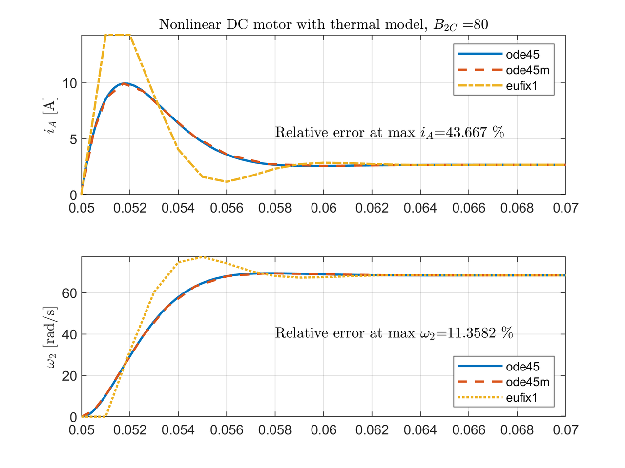
title(['Nonlinear DC motor with thermal model, $B_{2C}=$',num2str(B_2C)],'Interpreter','Latex');
ylabel('$i_A$ [A]','Interpreter','Latex');
legend('ode45','ode45m','eufix1');
axis([0.05 0.07 -inf inf]);
text(0.058,5.5,['Relative error at max $i_{A}$=',num2str(max_iA_error),' $\%$'],'Interpreter','Latex');
grid on;
subplot(2,1,2);
plot(t1,x1(:,2),t2,x2(:,2),'--',t3,x3(:,2),':','LineWidth',1.5);
ylabel('$\omega_2$ [rad/s]','Interpreter','Latex');
legend('ode45','ode45m','eufix1','Location','southeast');
axis([0.05 0.07 -inf inf]);
text(0.058,40,['Relative error at max $\omega_{2}$=',num2str(max_omega2_error),' $\%$'],'Interpreter','Latex');
grid on;
figure;
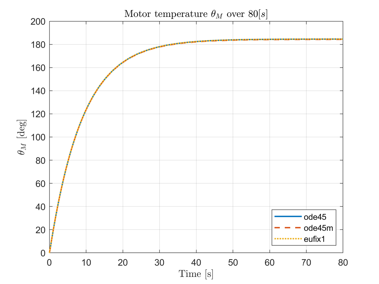
plot(t1,x1(:,3),t2,x2(:,3),'--',t3,x3(:,3),':','LineWidth',1.5);
title('Motor temperature $\theta_M$ over $80[s]$','Interpreter','Latex');
xlabel('Time [s]','Interpreter', 'Latex');
ylabel('$\theta_M$ [deg]','Interpreter','Latex');
legend('ode45','ode45m','eufix1','Location','southeast');
grid on;
elseif input_type == 1
%% Sinusoidal input e_i
figure;
subplot(3,1,1);
plot(t1,x1(:,1),t2,x2(:,1),'--',t3,x3(:,1),'-.','LineWidth',1.5);
title(['Nonlinear DC motor with thermal model, $B_{2C}=$',num2str(B_2C)],'Interpreter','Latex');
ylabel('$i_A$ [A]','Interpreter','Latex');
legend('ode45','ode45m','eufix1','Location','southeast');
grid on;
subplot(3,1,2);
plot(t1,x1(:,2),t2,x2(:,2),'--',t3,x3(:,2),':','LineWidth',1.5);
ylabel('$\omega_2$ [rad/s]','Interpreter','Latex');
legend('ode45','ode45m','eufix1','Location','southeast');
grid on;
subplot(3,1,3);
plot(t1,x1(:,3),t2,x2(:,3),'--',t3,x3(:,3),':','LineWidth',1.5);
xlabel('Time [s]','Interpreter', 'Latex');
ylabel('$\theta_M$ [deg]','Interpreter','Latex');
legend('ode45','ode45m','eufix1','Location','southeast');
grid on;
figure;
subplot(3,1,1);
plot(t1,x1(:,2),t2,x2(:,2),'--',t3,x3(:,2),'-.','LineWidth',1.5);
title(['Stiction behaviour on $\omega_2$, $B_{2C}=$',num2str(B_2C)],'Interpreter','Latex');
ylabel('$\omega_2$ [rad/s]','Interpreter','Latex');
legend('ode45','ode45m','eufix1','Location','southeast');
axis([0.148 0.157 -0.6 0.4]);
grid on;
subplot(3,1,2);
plot(t1,x1(:,2),t2,x2(:,2),'--',t3,x3(:,2),':','LineWidth',1.5);
ylabel('$\omega_2$ [rad/s]','Interpreter','Latex');
legend('ode45','ode45m','eufix1','Location','southeast');
axis([0.148 0.157 -0.015 0.010]);
grid on;
subplot(3,1,3);
plot(t1,x1(:,2),t2,x2(:,2),'--',t3,x3(:,2),'-.','LineWidth',1.5);
xlabel('Time [s]','Interpreter', 'Latex');
ylabel('$\omega_2$ [rad/s]','Interpreter','Latex');
legend('ode45','ode45m','eufix1','Location','southeast');
axis([0.148 0.157 -11e-5 5e-5]);
grid on;
figure;
plot(t1,x1(:,3),t2,x2(:,3),'--',t3,x3(:,3),':','LineWidth',1.5);
title('Motor temperature $\theta_M$ over $80[s]$','Interpreter','Latex');
xlabel('Time [s]','Interpreter', 'Latex');
ylabel('$\theta_M$ [deg]','Interpreter','Latex');
legend('ode45','ode45m','eufix1','Location','southeast');
grid on;
end


Simulation Scenarios
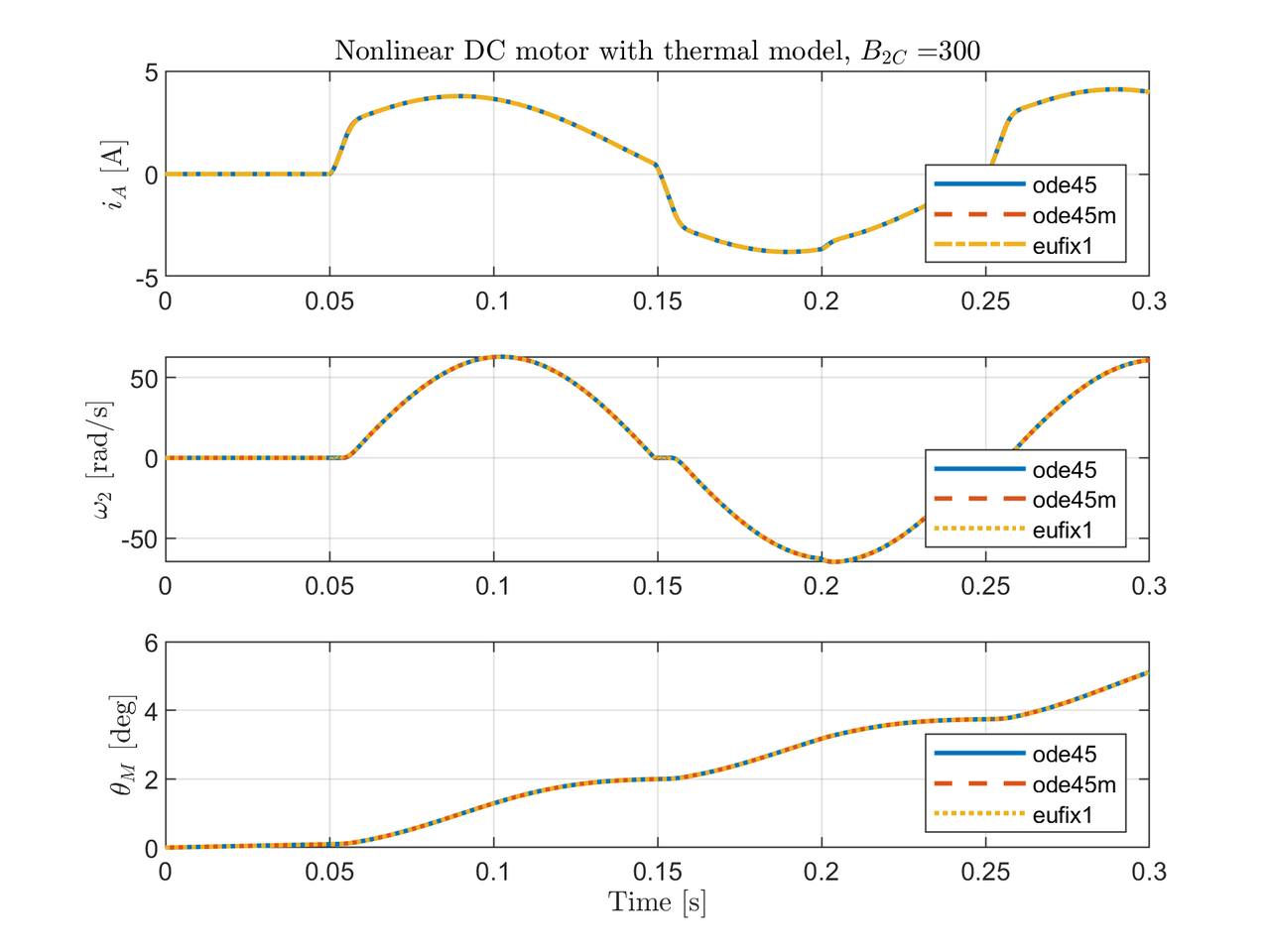
Two types of scenarios are simulated. The first one is submitted to a constant input, low stiction, and two step sizes. The second scenario is more interesting because we study the behaviour due to a sinusoidal input which emulates the reversing mode of the motor at $5[Hz]$ with higher stiction. Both scenarios have load torque at $t=0.2[s]$.
| Scenario 1 | Scenario 2 | |
|---|---|---|
ode45m step size |
$1\times 10^{-3}$ and $1\times 10^{-4}$ | $1\times 10^{-4}$ |
eufix1 step size |
$1\times 10^{-3}$ and $1\times 10^{-4}$ | $1\times 10^{-4}$ |
ode45 step size |
auto | auto |
| $e_i$ | $E_0$ | $E_0 \sin[5(2\pi)(t-0.05)]$ |
| $E_0$ | $120~[V]$ | $120~[V]$ |
| $\tau_{L}$ | $80~[N m]$ at $t=0.2[s]$} | $80~[N m]$ at $t=0.2[s]$ |
| $\theta_A$ | $18~[°C]$ | $18~[°C]$ |
| $B_{2C}$ | $80~[N]$ | $300~[N]$ |
Simulation Results
Scenario 1
The result in Fig. 1 shows the output states due to constant input $E_0=120$, and $B_{2C}=80$. The current overshoot at $0.05[s]$ is due to the inertia that the motor has to overcome. After the inertia is broken, the current $i_A$ drops down to a constant value. The load torque $\tau_{L}$ is applied at $0.2[s]$ which produces the increment in the current and the decrement in the angular velocity. Also, eufix1 solves the system with noticeable error, this result is analyzed later.
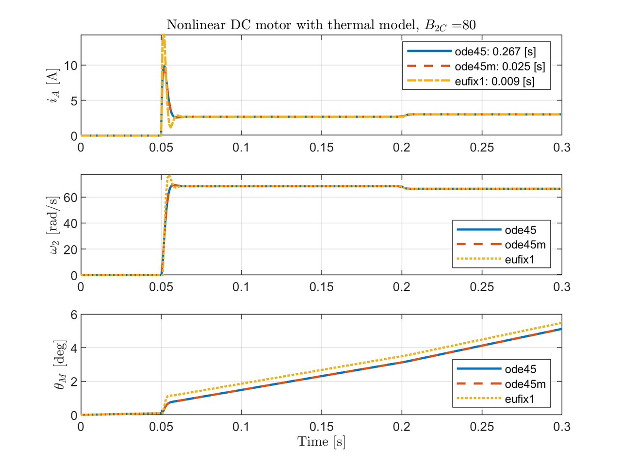
The time simulation of each solver indicates that ode45 is 10 times slower than ode45m and 30 times slower than eufix1.
ode45 |
ode45m |
eufix1 |
|
|---|---|---|---|
| simulation time [s] | $0.267$ | $0.025$ | $0.009$ |
| number of time steps | $71769$ | $15133$ | $80001$ |
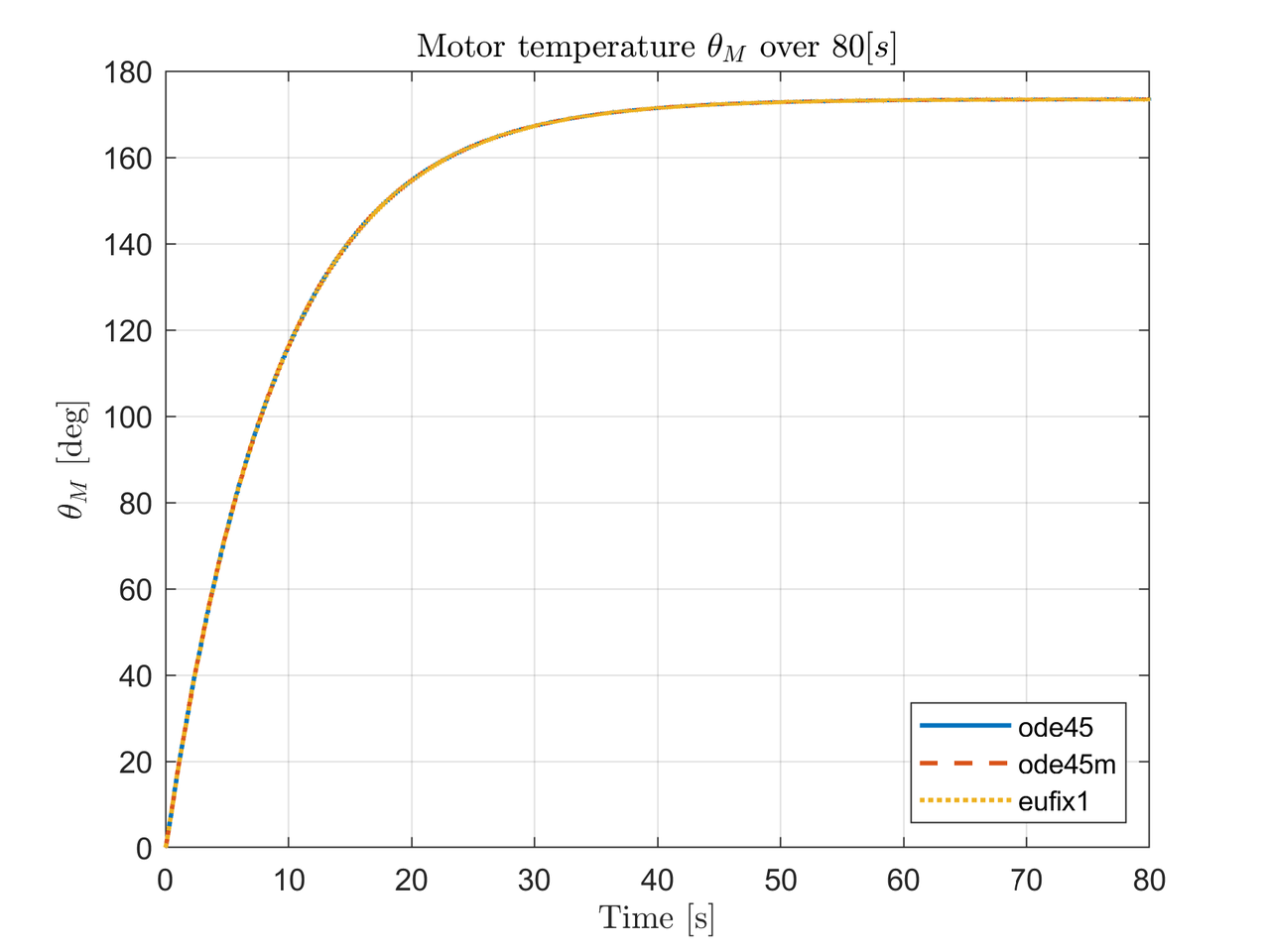
The temperature of the motor $\theta_M$ increases linearly and reaches steady-state at $45[s]$ approximately, which indicates that the motor won't reach unsafe temperatures.
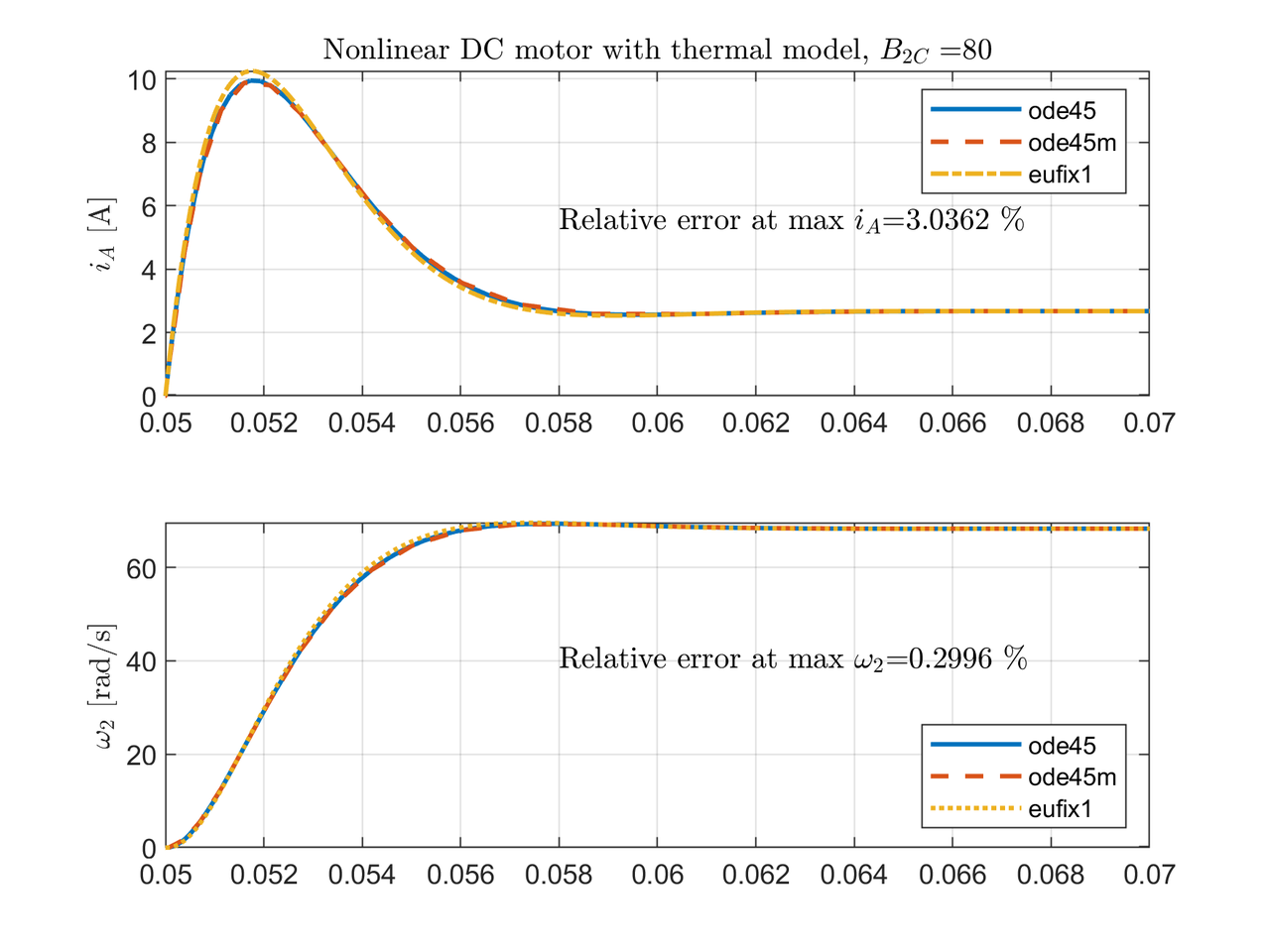
Although, eufix1 is the fastest solver, with step size of $1\times 10^{-3}$, eufix1 outputs the worst performance. The result can be improved if the steps size is decreased to $1\times 10^{-4}$. Fig. 3 and Fig. 4 show the relative error at max current and max angular velocity between ode45 and eufix1.
Scenario 2
In this scenario we submitted the DC motor to high stiction $B_{2C}=300$ and sinsusoidal input at $5[Hz]$ which simulates the reversing mode. Table 3 shows the output for the three solvers showing that ode45 is the slowest by far.
ode45 |
ode45m |
eufix1 |
|
|---|---|---|---|
| simulation time [s] | $517.798$ | $3.463$ | $0.093$ |
| number of time steps | $13559913$ | $9647$ | $3002$ |
Fig. 5 shows the simulation output. The relevant result is the behavior of the system around the (nonlinear) stiction. $\omega_2$ sticks at $0.15[s]$ and $0.25[s]$ due to $B_{2C}$.
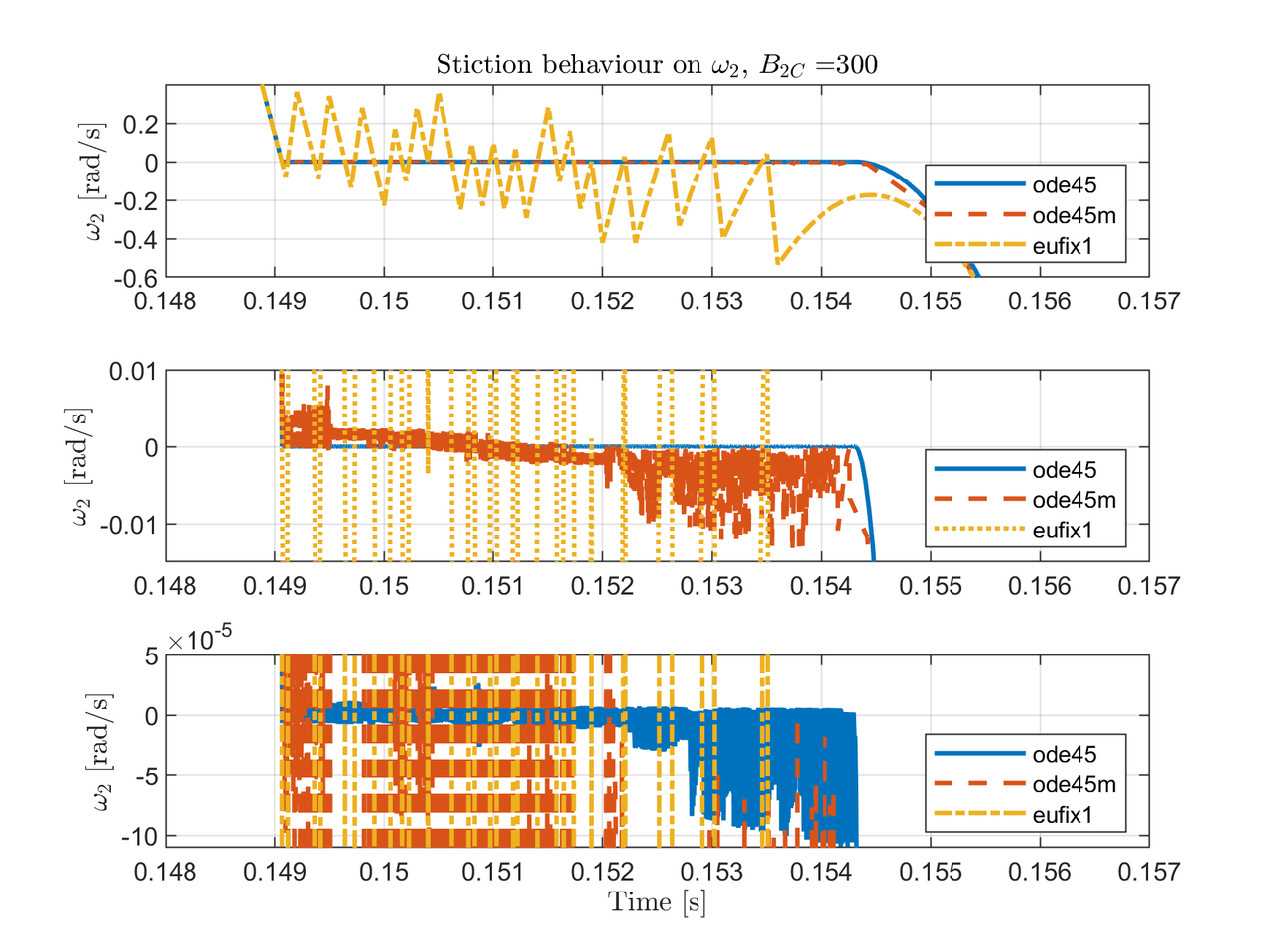
Even though the solvers were able to solve the dynamics with stiction, ode45 took too much time to overcome this nonlinearity. Fig. 6 shows the stiction with three different zoom levels for each solver. The fastest but with more integration step error is eufix1. ode45m has less error $\pm 0.01$, and finally ode45 solves with the minimum error, around $\pm 10\times 10^{-5}$. In conclusion, ode45m is the best choice against the rest because it can obtain the solution with low error and with decent speed.
The motor temperature $\theta_M$ in reversing mode reaches the steady-state at $45[s]$ approximately which indicates the motor won't suffer overheat due to stiction.
Comments
Comments powered by Disqus